Chapter 1: Introduction to the Chernoff Bound

In this section, we explore the concept of the Chernoff Bound and its relevance in understanding the behavior of random variables. Imagine tossing n fair coins sequentially and counting the number of HEADS, represented as X. What can we infer about the value of X? This inquiry serves as the focal point of our discussion.

To begin, we label the coins from 1 to n and define a random variable (X_i) that equals 1 if the i-th coin toss results in HEADS and 0 otherwise. It's evident that for each i from 1 to n, the probability of (X_i = 1) is (1/2). This leads us to the equation:

[X = X_1 + X_2 + ... + X_n]

The next step is to calculate the expected value of X using a property known as Linearity of Expectation. This principle states that the expected value of a sum of random variables (regardless of their independence) equals the sum of their expected values. Therefore, we can express:

[E[X] = E[X_1 + X_2 + ... + X_n] = E[X_1] + E[X_2] + ... + E[X_n] = frac{n}{2}]

This indicates that the anticipated number of HEADS is (n/2). While this result is satisfying, it prompts a further question: What is the likelihood of X being "close enough" to this expected value? Specifically, we ask:

What is the probability that X approximates its expected value?

To address this, we will employ the renowned Chernoff Bound, defined as follows:

The Chernoff Bound, named after Herman Chernoff, provides exponentially decreasing bounds on the tail distributions of sums of independent random variables. This bound is more precise than the traditional tail bounds derived from the first or second moments, such as Markov's or Chebyshev's inequalities.

The first video titled "6. Concentration Inequalities: The Chernoff Bound" explains the concept in detail, showcasing its derivation and implications.

What Exactly is the Chernoff Bound?

In essence, the Chernoff Bound offers robust concentration results for sums of independent random variables. Our focus will be on sums of 0/1 random variables, specifically within the context we have established. We aim to demonstrate a strong concentration around the expected value, examining the probabilities of the following events:

[Pleft[X geq (1 + delta) muright]] [Pleft[X leq (1 - delta) muright]]

where (delta > 0) is a small real number, and (mu = E[X] = n/2) denotes the expected value of X.

Before proceeding, we state Markov's Inequality:

Markov's Inequality: Let X be a non-negative random variable and A be a positive real number. Then:

[P[X geq A] leq frac{E[X]}{A}]

We introduce a positive parameter (t > 0), which will be defined later, and express:

Applying Markov's Inequality yields:

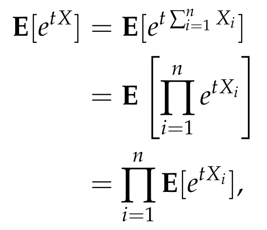
Next, we analyze the numerator on the right side:

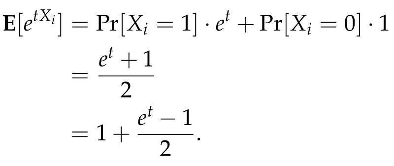
Each term in this product can be computed easily. We utilize the inequality (1 + x leq e^x), leading to:

Consequently, we derive:

Integrating all parts, we conclude:

To minimize the right side, we focus on minimizing the exponent since (t > 0) is a free parameter. The exponential function's strictly increasing nature implies minimizing the exponent leads us to:

The first derivative of this function is:

This indicates that the function reaches its minimum at (t = ln(1 + delta)). Substituting this value yields:

Thus, we arrive at the Chernoff Bound!

The second video titled "Proof of the Chernoff Bound" from CMU provides a comprehensive lecture on deriving this bound, enhancing our understanding.

Simplifying the Chernoff Bound

While the expression above may seem complex, we can obtain a simpler, albeit slightly looser, bound through additional analysis.

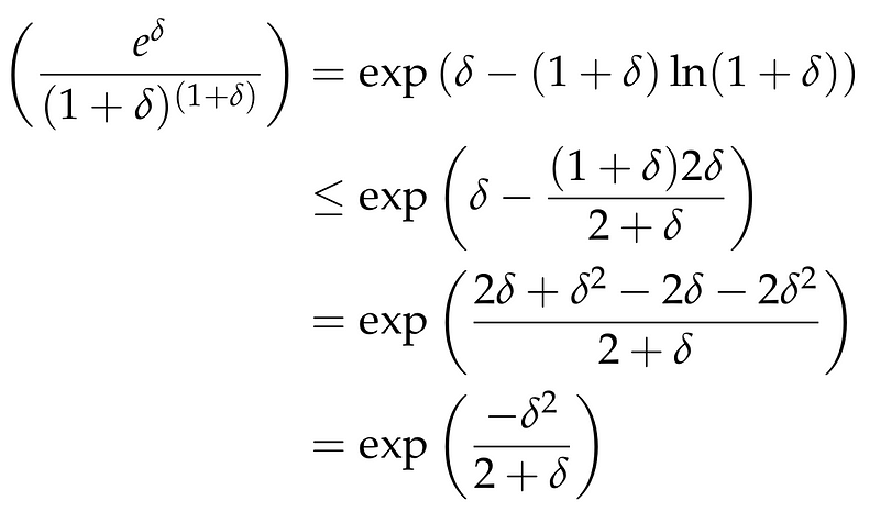
Returning to the right side of the Chernoff bound, we can express it as follows:

This leads us to a generalized form of the Chernoff Bound that holds for any (delta > 0):

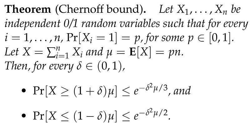
By focusing on smaller values of (delta), particularly when (0 < delta < 1), we can derive the following form of the Chernoff Bound:

This theorem generalizes our discussion in two ways: Firstly, it allows for biased coin flips where each coin has a probability (p) of landing HEADS, with (p) in the range [0,1]. Secondly, it can also provide bounds for the probability that X falls below ((1 - delta)mu).

Returning to our initial inquiry, we can now apply this theorem to conclude:

This analysis shows that as the number of coins (n) increases, the probability of deviating from the expected value decreases exponentially. Essentially, the majority of the random variable X is concentrated within a narrow interval around the expected value, a result far more robust than what can be achieved through Markov's or Chebyshev's inequalities.

Conclusion

The phenomenon of concentration of measure is invaluable across various fields such as statistics, randomized algorithms, and machine learning. One particularly elegant application of this concept relates to dimensionality reduction in Euclidean spaces. The Chernoff Bound serves as a crucial tool in quantifying this concentration, appearing in numerous practical applications. By utilizing Chernoff bounds, we can assert that our estimates are closely aligned with the true values and that algorithms perform successfully with high probability.

Chernoff bounds can even be established for cases where random variables are not independent, but perhaps negatively correlated. The study of concentration of measure theory is extensive, and interested readers are encouraged to delve into available resources online.

In summary, Chernoff bounds are extraordinarily beneficial and applicable in numerous contexts, making them an essential concept to remember!